

Changes In The Price Level Affect Which Components Of Aggregate Demand?
The Aggregate Need/Aggregate Supply Model
Building a Model of Amass Demand and Aggregate Supply
Learning Objectives
By the terminate of this section, yous volition be able to:
- Explicate the aggregate supply curve and how information technology relates to real GDP and potential GDP
- Explicate the aggregate demand curve and how it is influenced past price levels
- Interpret the aggregate demand/aggregate supply model
- Identify the point of equilibrium in the aggregate demand/aggregate supply model
- Define curt run aggregate supply and long run aggregate supply
To build a useful macroeconomic model, we need a model that shows what determines total supply or total need for the economy, and how total demand and total supply collaborate at the macroeconomic level. Nosotros telephone call this the aggregate demand/aggregate supply model. This module volition explain aggregate supply, aggregate need, and the equilibrium between them. The post-obit modules will hash out the causes of shifts in aggregate supply and amass demand.
The Aggregate Supply Curve and Potential GDP
Firms brand decisions about what quantity to supply based on the profits they expect to earn. They decide profits, in turn, past the price of the outputs they sell and past the prices of the inputs, like labor or raw materials, that they demand to buy. Aggregate supply (Every bit) refers to the total quantity of output (i.e. real Gross domestic product) firms volition produce and sell. The aggregate supply (Equally) curve shows the full quantity of output (i.e. real GDP) that firms will produce and sell at each price level.
[link] shows an aggregate supply curve. In the post-obit paragraphs, we will walk through the elements of the diagram one at a time: the horizontal and vertical axes, the aggregate supply curve itself, and the pregnant of the potential Gdp vertical line.

The diagram's horizontal axis shows existent Gdp—that is, the level of Gdp adjusted for inflation. The vertical axis shows the cost level, which measures the average price of all goods and services produced in the economy. In other words, the price level in the AD-Equally model is what we called the Gross domestic product Deflator in The Macroeconomic Perspective. Remember that the cost level is dissimilar from the inflation rate. Visualize the cost level as an alphabetize number, like the Consumer Price Index, while the aggrandizement rate is the pct change in the price level over time.
As the price level rises, real GDP rises as well. Why? The price level on the vertical axis represents prices for final goods or outputs bought in the economy—i.eastward. the GDP deflator—not the cost level for intermediate goods and services that are inputs to production. Thus, the AS bend describes how suppliers will react to a higher toll level for final outputs of goods and services, while property the prices of inputs like labor and energy constant. If firms across the economy face a situation where the price level of what they produce and sell is ascension, only their costs of production are not ascent, then the lure of higher profits volition induce them to expand production. In other words, an aggregate supply curve shows how producers as a group will respond to an increment in aggregate demand.
An AS bend's slope changes from almost flat at its far left to nearly vertical at its far right. At the far left of the aggregate supply bend, the level of output in the economy is far below potential Gross domestic product, which we define equally the amount of real Gross domestic product an economy can produce by fully employing its existing levels of labor, physical capital letter, and engineering science, in the context of its existing market place and legal institutions. At these relatively low levels of output, levels of unemployment are loftier, and many factories are running only part-time, or have airtight their doors. In this situation, a relatively small increase in the prices of the outputs that businesses sell—while bold no rise in input prices—tin can encourage a considerable surge in the quantity of aggregate supply considering so many workers and factories are ready to swing into production.
Equally the GDP increases, yet, some firms and industries volition get-go running into limits: perhaps almost all of the expert workers in a certain manufacture will have jobs or factories in certain geographic areas or industries will be running at full speed. In the AS bend's intermediate area, a higher price level for outputs continues to encourage a greater quantity of output—but as the increasingly steep upward slope of the aggregate supply bend shows, the increase in existent GDP in response to a given rise in the price level volition not be as big. (Read the following Clear Information technology Upwardly feature to learn why the Every bit curve crosses potential Gross domestic product.)
Why does Equally cross potential Gdp?
Economists typically draw the aggregate supply curve to cross the potential GDP line. This shape may seem puzzling: How tin an economy produce at an output level which is higher than its "potential" or "full employment" Gross domestic product? The economical intuition here is that if prices for outputs were high plenty, producers would make fanatical efforts to produce: all workers would be on double-overtime, all machines would run 24 hours a day, vii days a week. Such hyper-intense production would go beyond using potential labor and physical capital resources fully, to using them in a style that is not sustainable in the long term. Thus, information technology is possible for production to sprint to a higher place potential GDP, merely simply in the short run.
At the far correct, the aggregate supply curve becomes nearly vertical. At this quantity, college prices for outputs cannot encourage boosted output, because fifty-fifty if firms desire to expand output, the inputs of labor and mechanism in the economy are fully employed. In this example, the vertical line in the showroom shows that potential Gdp occurs at a total output of 9,500. When an economic system is operating at its potential Gdp, machines and factories are running at capacity, and the unemployment rate is relatively low—at the natural rate of unemployment. For this reason, potential GDP is sometimes also called total-employment Gross domestic product.
The Aggregate Demand Curve
Aggregate demand (AD) refers to the corporeality of total spending on domestic appurtenances and services in an economy. (Strictly speaking, Advert is what economists phone call full planned expenditure. Nosotros volition farther explicate this stardom in the appendix The Expenditure-Output Model
. For now, simply think of aggregate demand as total spending.) It includes all iv components of demand: consumption, investment, government spending, and net exports (exports minus imports). This demand is determined by a number of factors, but one of them is the price level—recall though, that the price level is an index number such as the Gross domestic product deflator that measures the average price of the things nosotros buy. The aggregate demand (AD) curve shows the total spending on domestic appurtenances and services at each price level.
[link] presents an amass demand (AD) curve. Simply like the aggregate supply curve, the horizontal axis shows real Gross domestic product and the vertical axis shows the toll level. The AD curve slopes down, which means that increases in the price level of outputs lead to a lower quantity of total spending. The reasons behind this shape are related to how changes in the price level affect the different components of amass need. The following components contain aggregate demand: consumption spending (C), investment spending (I), authorities spending (G), and spending on exports (X) minus imports (M): C + I + G + X – G.

The wealth event holds that as the price level increases, the buying power of savings that people have stored up in banking concern accounts and other assets will diminish, eaten away to some extent by inflation. Because a rise in the price level reduces people'due south wealth, consumption spending will fall equally the cost level rises.
The interest rate effect is that as prices for outputs rise, the same purchases will have more money or credit to accomplish. This additional demand for money and credit will push involvement rates higher. In plow, higher interest rates volition reduce borrowing by businesses for investment purposes and reduce borrowing by households for homes and cars—thus reducing consumption and investment spending.
The strange price effect points out that if prices rise in the United States while remaining stock-still in other countries, and then goods in the United States will exist relatively more than expensive compared to goods in the residuum of the world. U.S. exports volition exist relatively more expensive, and the quantity of exports sold will autumn. U.S. imports from abroad will be relatively cheaper, and so the quantity of imports will rise. Thus, a higher domestic price level, relative to price levels in other countries, volition reduce internet consign expenditures.
Amidst economists all three of these effects are controversial, in part considering they do not seem to exist very large. For this reason, the amass demand curve in [link] slopes downwards adequately steeply. The steep gradient indicates that a higher cost level for final outputs reduces amass need for all three of these reasons, but that the change in the quantity of amass demand as a result of changes in cost level is non very large.
Read the post-obit Work Information technology Out feature to learn how to interpret the Advert/As model. In this instance, aggregate supply, aggregate demand, and the price level are given for the imaginary country of Xurbia.
Interpreting the AD/As Model
[link] shows information on amass supply, aggregate demand, and the toll level for the imaginary country of Xurbia. What information does [link] tell yous almost the land of the Xurbia's economy? Where is the equilibrium price level and output level (this is the SR macroequilibrium)? Is Xurbia risking inflationary pressures or facing high unemployment? How can y'all tell?
| Price Level | Amass Demand | Aggregate Supply |
|---|---|---|
| 110 | $700 | $600 |
| 120 | $690 | $640 |
| 130 | $680 | $680 |
| 140 | $670 | $720 |
| 150 | $660 | $740 |
| 160 | $650 | $760 |
| 170 | $640 | $770 |
To brainstorm to use the Advertisement/Every bit model, it is important to plot the Every bit and AD curves from the data provided. What is the equilibrium?
Stride one. Draw your x- and y-centrality. Label the ten-axis Real Gross domestic product and the y-centrality Price Level.
Pace two. Plot Advert on your graph.
Stride 3. Plot Every bit on your graph.
Footstep 4. Look at [link] which provides a visual to aid in your assay.

Stride 5. Determine where Advertising and Every bit intersect. This is the equilibrium with price level at 130 and real GDP at $680.
Step 6. Await at the graph to determine where equilibrium is located. We can see that this equilibrium is fairly far from where the AS bend becomes nigh-vertical (or at to the lowest degree quite steep) which seems to start at about $750 of real output. This implies that the economy is not shut to potential GDP. Thus, unemployment volition be high. In the relatively apartment part of the AS bend, where the equilibrium occurs, changes in the price level will non be a major concern, since such changes are likely to be modest.
Step 7. Make up one's mind what the steep portion of the AS curve indicates. Where the AS curve is steep, the economy is at or close to potential Gdp.
Stride viii. Draw conclusions from the given information:
- If equilibrium occurs in the flat range of AS, then economy is not close to potential Gross domestic product and will be experiencing unemployment, only stable price level.
- If equilibrium occurs in the steep range of AS, then the economy is close or at potential Gross domestic product and will be experiencing rising price levels or inflationary pressures, only volition have a low unemployment rate.
Equilibrium in the Aggregate Need/Aggregate Supply Model
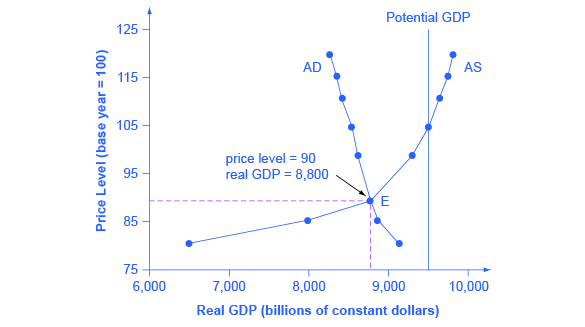
The intersection of the amass supply and aggregate demand curves shows the equilibrium level of existent Gdp and the equilibrium price level in the economy. At a relatively low price level for output, firms have piddling incentive to produce, although consumers would exist willing to purchase a large quantity of output. Equally the price level rises, aggregate supply rises and aggregate demand falls until the equilibrium point is reached.
[link] combines the Every bit bend from [link] and the AD curve from [link] and places them both on a single diagram. In this case, the equilibrium signal occurs at point E, at a price level of 90 and an output level of 8,800.
Confusion sometimes arises between the amass supply and amass demand model and the microeconomic analysis of demand and supply in particular markets for appurtenances, services, labor, and capital. Read the post-obit Clear It Up feature to gain an understanding of whether AS and Advertizing are macro or micro.
Are AS and Ad macro or micro?
These aggregate supply and need models and the microeconomic assay of demand and supply in particular markets for goods, services, labor, and capital letter have a superficial resemblance, only they also have many underlying differences.
For example, the vertical and horizontal axes have distinctly unlike meanings in macroeconomic and microeconomic diagrams. The vertical centrality of a microeconomic demand and supply diagram expresses a price (or wage or charge per unit of render) for an individual proficient or service. This price is implicitly relative: information technology is intended to exist compared with the prices of other products (for example, the price of pizza relative to the cost of fried craven). In dissimilarity, the vertical axis of an aggregate supply and aggregate need diagram expresses the level of a cost alphabetize like the Consumer Toll Index or the Gross domestic product deflator—combining a wide array of prices from across the economy. The cost level is accented: information technology is not intended to be compared to whatsoever other prices since it is essentially the average price of all products in an economy. The horizontal axis of a microeconomic supply and need curve measures the quantity of a particular skilful or service. In contrast, the horizontal centrality of the aggregate demand and aggregate supply diagram measures GDP, which is the sum of all the terminal goods and services produced in the economic system, not the quantity in a specific market.
In addition, the economic reasons for the shapes of the curves in the macroeconomic model are unlike from the reasons behind the shapes of the curves in microeconomic models. Demand curves for individual goods or services slope downwards primarily because of the being of substitute goods, not the wealth effects, interest rate, and foreign price effects associated with amass demand curves. The slopes of private supply and demand curves can have a variety of dissimilar slopes, depending on the extent to which quantity demanded and quantity supplied react to price in that specific marketplace, but the slopes of the Every bit and AD curves are much the same in every diagram (although as nosotros shall come across in later chapters, curt-run and long-run perspectives will emphasize different parts of the As bend).
In short, only considering the Advertizement/AS diagram has ii lines that cross, exercise not assume that it is the same equally every other diagram where ii lines cross. The intuitions and meanings of the macro and micro diagrams are simply distant cousins from different branches of the economics family tree.
Defining SRAS and LRAS
In the Clear It Up characteristic titled "Why does Every bit cross potential Gross domestic product?" we differentiated between curt run changes in amass supply which the AS bend shows and long run changes in amass supply which the vertical line at potential GDP defines. In the brusk run, if demand is too low (or also loftier), it is possible for producers to supply less Gdp (or more Gross domestic product) than potential. In the long run, all the same, producers are limited to producing at potential Gdp. For this reason, we may also refer to what we take been calling the AS bend equally the short run aggregate supply (SRAS) bend. We may as well refer to the vertical line at potential Gdp equally the long run aggregate supply (LRAS) bend.
Key Concepts and Summary
The up-sloping curt run aggregate supply (SRAS) curve shows the positive relationship between the toll level and the level of existent GDP in the short run. Aggregate supply slopes upwards because when the cost level for outputs increases, while the price level of inputs remains fixed, the opportunity for additional profits encourages more than product. The aggregate supply curve is near-horizontal on the left and near-vertical on the correct. In the long run, nosotros show the amass supply by a vertical line at the level of potential output, which is the maximum level of output the economy can produce with its existing levels of
workers, physical majuscule, technology, and economic institutions.
The downward-sloping aggregate demand (Advert) bend shows the human relationship between the toll level for outputs and the quantity of total spending in the economy. It slopes downward because of: (a) the wealth effect, which means that a higher price level leads to lower real wealth, which reduces the level of consumption; (b) the interest charge per unit issue, which holds that a higher price level will mean a greater demand for money, which will tend to drive up interest rates and reduce investment spending; and (c) the strange price consequence, which holds that a rise in the price level will make domestic goods relatively more expensive, discouraging exports and encouraging imports.
Self-Cheque Questions
The brusque run amass supply bend was constructed assuming that as the toll of outputs increases, the toll of inputs stays the same. How would an increase in the prices of important inputs, similar energy, bear on aggregate supply?
[reveal-reply q="349873″]Show Solution[/reveal-reply]
[hidden-respond a="349873″]Higher input prices make output less assisting, decreasing the desired supply. This is shown graphically every bit a leftward shift in the Equally bend.[/hidden-reply]
In the Advert/As model, what prevents the economy from achieving equilibrium at potential output?
[reveal-respond q="104967″]Show Solution[/reveal-answer]
[hidden-respond a="104967″]Equilibrium occurs at the level of Gross domestic product where Advertizing = Equally. Bereft aggregate demand could explain why the equilibrium occurs at a level of GDP less than potential. A decrease (or leftward shift) in aggregate supply could be another reason.[/subconscious-answer]
Review Questions
What is on the horizontal axis of the Advert/Equally diagram? What is on the vertical axis?
What is the economic reason why the SRAS curve slopes up?
What are the components of the aggregate demand (Advert) curve?
What are the economic reasons why the Advertising bend slopes down?
Briefly explain the reason for the near-horizontal shape of the SRAS curve on its far left.
Briefly explain the reason for the near-vertical shape of the SRAS curve on its far right.
Critical Thinking Questions
On a microeconomic demand bend, a decrease in toll causes an increase in quantity demanded because the product in question is now relatively less expensive than substitute products. Explicate why amass demand does not increment for the aforementioned reason in response to a decrease in the aggregate cost level. In other words, what causes full spending to increase if it is not because goods are now cheaper?
Problems
Review the trouble in the Piece of work Information technology Out titled "Interpreting the AD/Equally Model." Similar the information provided in that feature, [link] shows data on aggregate supply, aggregate need, and the price level for the imaginary land of Xurbia.
| Cost Level | AD | Every bit |
|---|---|---|
| 110 | 700 | 600 |
| 120 | 690 | 640 |
| 130 | 680 | 680 |
| 140 | 670 | 720 |
| 150 | 660 | 740 |
| 160 | 650 | 760 |
| 170 | 640 | 770 |
- Plot the AD/AS diagram from the data. Identify the equilibrium.
- Imagine that, as a result of a government taxation cut, amass demand becomes higher by 50 at every cost level. Identify the new equilibrium.
- How volition the new equilibrium modify output? How will information technology alter the price level? What do you think volition happen to employment?
The imaginary country of Harris Island has the aggregate supply and aggregate demand curves equally [link] shows.
| Price Level | Advertising | As |
|---|---|---|
| 100 | 700 | 200 |
| 120 | 600 | 325 |
| 140 | 500 | 500 |
| 160 | 400 | 570 |
| 180 | 300 | 620 |
- Plot the AD/Every bit diagram. Identify the equilibrium.
- Would you await unemployment in this economy to be relatively high or low?
- Would yous await business about aggrandizement in this economy to be relatively high or low?
- Imagine that consumers brainstorm to lose confidence nigh the land of the economy, and then AD becomes lower by 275 at every cost level. Identify the new amass equilibrium.
- How will the shift in AD affect the original output, cost level, and employment?
[link] describes Santher'south economy.
| Price Level | AD | Equally |
|---|---|---|
| 50 | 1,000 | 250 |
| 60 | 950 | 580 |
| 70 | 900 | 750 |
| 80 | 850 | 850 |
| ninety | 800 | 900 |
- Plot the Ad/AS curves and place the equilibrium.
- Would you lot expect unemployment in this economy to be relatively loftier or depression?
- Would you expect prices to be a relatively big or small-scale concern for this economy?
- Imagine that input prices fall and then AS shifts to the right by 150 units. Place the new equilibrium.
- How volition the shift in AS touch on the original output, toll level, and employment?
Glossary
- aggregate need (Advertising)
- the amount of total spending on domestic goods and services in an economy
- aggregate supply (AS)
- the total quantity of output (i.east. real GDP) firms volition produce and sell
- aggregate need (AD) curve
- the total spending on domestic goods and services at each price level
- aggregate supply (AS) curve
- the total quantity of output (i.due east. existent Gross domestic product) that firms will produce and sell at each price level
- amass need/aggregate supply model
- a model that shows what determines total supply or full demand for the economy, and how full need and total supply interact at the macroeconomic level
- full-employment Gross domestic product
- another proper name for potential Gdp, when the economy is producing at its potential and unemployment is at the natural rate of unemployment
- long run amass supply (LRAS) curve
- vertical line at potential GDP showing no human relationship between the price level for output and real Gdp in the long run
- potential GDP
- the maximum quantity that an economy can produce given full employment of its existing levels of labor, physical capital, technology, and institutions
- short run aggregate supply (SRAS) curve
- positive short run human relationship betwixt the price level for output and real Gdp, holding the prices of inputs fixed

Source: https://opentextbc.ca/macroeconomics2eopenstax/chapter/building-a-model-of-aggregate-demand-and-aggregate-supply/
Posted by: hancockhitylo.blogspot.com
0 Response to "Changes In The Price Level Affect Which Components Of Aggregate Demand?"
Post a Comment